CryoGEN-I: MAP estimation under an energy prior

Reconstruct each degraded tomogram into its single most probable clean volume — with an energy prior and the $P_Y$ proxy, and no ground truth at all

CryoGEN-I is the starting point of the CryoGEN lineage: it takes a tomogram $y$ corrupted by noise and the missing wedge and reconstructs the single most probable clean volume $x$ it corresponds to — a MAP (maximum a posteriori) point estimate, with no ground-truth labels at all. It gives the lineage its simplest and most rigorous foundation; CryoGEN-II then lifts “per-image optimality” to global distribution matching, and CryoWGEN replaces the single answer with a whole family of reconstructions.

Intuition

CryoGEN-I asks the most basic question: for each $y$ , what is the single most probable reconstruction $x$ ? That is a MAP problem. The catch is not the solving but the unseen prior $p(x)$ : we have no labels for clean volumes, and no formula for the density of “what makes an $x$ look like real structure.”

The way out rests on one observation: if a guessed reconstruction $x$ is plausible, then rotating it by a random angle and re-applying the missing-wedge corruption should produce something that looks just like a real, observed tomogram. If the corrupted result looks unlike any real data, $x$ must be wrong. Real data is abundant — so “does it look like a real observation?” becomes the supervision signal. This is CryoGEN’s $P_Y$ proxy idea.

The imaging model: turning unsupervised into matching in observation space

The whole CryoGEN lineage builds on the same degradation model:

y = \mathcal{T}_M(x) + \epsilon_n, \qquad \epsilon_n \sim \mathcal{N}(0, \sigma_n^2 I)

Term by term: $x$ is the isotropic clean volume we want; $\mathcal{T}_M$ is the missing-wedge operator, which carves out the wedge of Fourier space outside the tilt range — exactly what stretches a tomogram anisotropically along the missing direction; $\epsilon_n$ is Gaussian noise of variance $\sigma_n^2$ ; and $y$ is the corrupted observation, the only thing we actually hold.

The key is to add a random rotation $R$ . The composite operator $\mathcal{T}_M \circ R$ bridges the “clean reconstruction space $\mathcal{X}$ ” and the “observed space $\mathcal{Y}$ ”: take any candidate $x$ , rotate it to a random orientation, apply the missing wedge, and you have projected it into observation space — where abundant real data is available to compare against. This bridge is what makes unsupervised learning possible: it translates “a reconstruction problem with no labels” into “does this match the real distribution in observation space?”

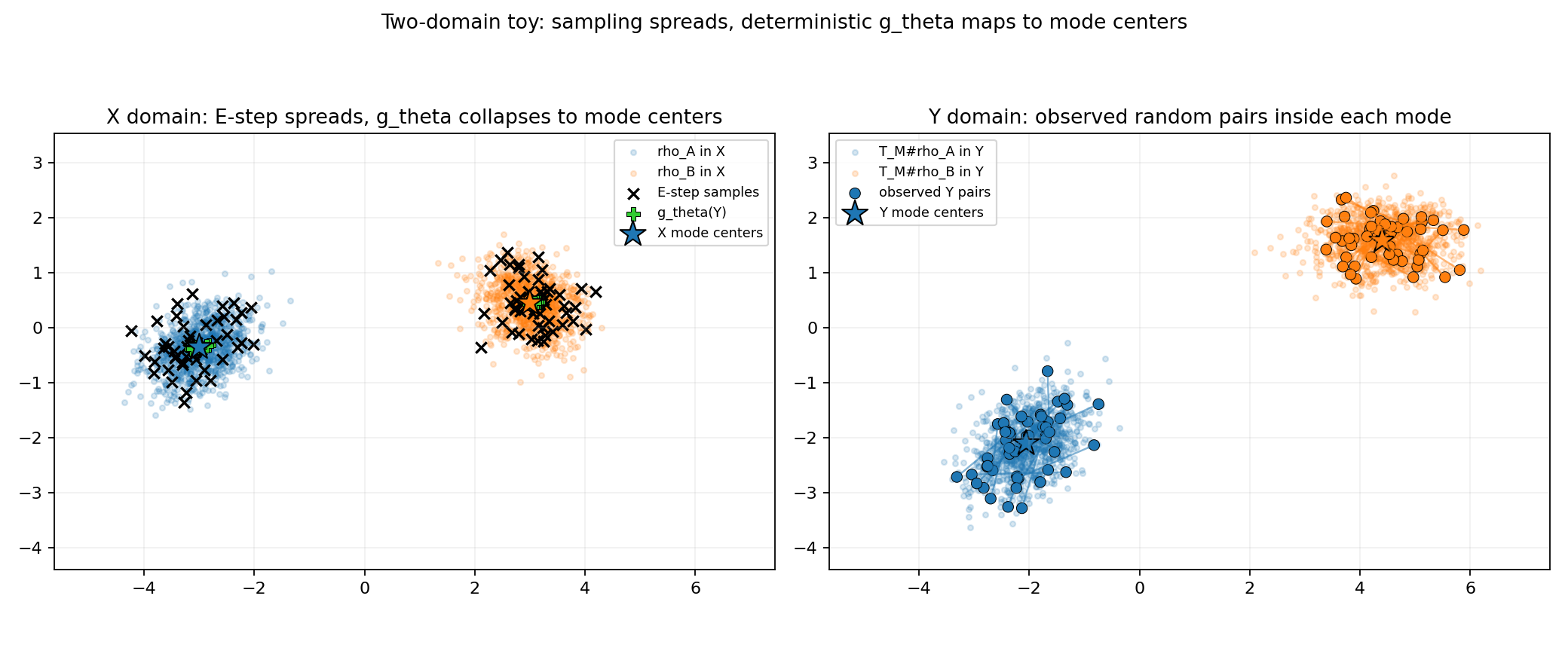
Two-domain toy example of the X and Y spaces — Two-domain toy example: left is the reconstruction space X, where E-step samples spread out and the network g_θ collapses them to the mode centers; right is the observation space Y with paired real samples. Training alternates EM-style — the E-step samples candidate restorations, the M-step updates network parameters, and the discriminator (D-step) supplies the adversarial prior.

The energy prior: learning “plausible” as a scalar function

MAP needs the prior $p(x)$ , which we cannot write down. CryoGEN-I parameterizes it as an energy function $E_\phi(x)$ — a scalar network that scores a volume $x$ , where lower energy = more plausible. The bridge from energy to probability is the Boltzmann form:

p(x) = \frac{1}{Z}\exp\!\big(-E_\phi(x)\big)

Here $E_\phi(x)$ is the energy with parameters $\phi$ ; the exponential turns “low energy” into “high probability”; and $Z=\int e^{-E_\phi(x)}\,dx$ is the partition function, which integrates over all $x$ to normalize the density. The local minima of the energy are the modes of the density — to see how an energy function shapes its density, and how the depth of a well decides where probability mass concentrates, drag the one-dimensional example below:

Energy E(x)Density p(x) ∝ exp(−E(x)/T)

Well separation d: 4.0Temperature T: 1.00

Lower energy means higher probability: the two well bottoms become the two peaks of the density. Higher T flattens exp(−E/T), pushing the density toward uniform and erasing the contrast between the wells.

Depth

$Z$ is a high-dimensional integral and intractable. But this is precisely where MAP helps: it only compares the energies of different $x$ and never needs $Z$ — because $Z$ is the same constant for every $x$ , it cancels in the $\arg\min$ .

So how is $E_\phi$ trained? Here the $P_Y$ proxy does its second job: the energy can be trained entirely in observation space. Train a discriminator to tell real observations $y$ apart from corrupted reconstructions $\mathcal{T}_M\circ R(x)$ ; the boundary it learns is implicitly an energy separating plausible from implausible $x$ — an implausible $x$ does not look like real data once corrupted, so it is pushed to high energy. The prior never touches a single ground-truth label.

The MAP objective: balancing data fidelity against the energy prior

Putting the two pieces together, the MAP estimate is an optimization regularized by the prior:

x^* = \arg\min_{x}\; \frac{1}{2\sigma_n^2}\big\|\mathcal{T}_M(x)-y\big\|_2^2 \;+\; E_\phi(x)

The first term is data fidelity: once a candidate $x$ is corrupted ( $\mathcal{T}_M(x)$ ) it must match the observation $y$ in hand, with the mismatch weighted by $1/\sigma_n^2$ — the smaller the noise, the stricter this term. The second term is the energy prior: among all $x$ that explain the observation equally well, it pulls the solution toward the low-energy one, the one that most resembles real structure. The information the missing wedge erased is restored exactly through this second term — data fidelity has nothing to say about the missing frequencies inside the wedge, so the prior chooses for it.

Depth

Why is this the right weighting? For Gaussian noise $\epsilon_n\sim\mathcal{N}(0,\sigma_n^2 I)$ , the likelihood is $p(y\mid x)\propto\exp\!\big(-\tfrac{1}{2\sigma_n^2}\|\mathcal{T}_M(x)-y\|_2^2\big)$ . Multiply it by the prior $p(x)\propto e^{-E_\phi(x)}$ , take the negative log, and the constant terms (containing $Z$ and $\sigma_n$ ) are independent of $x$ and drop out — what remains is exactly the sum above. So CryoGEN-I is not an ad-hoc sum of two terms but the precise form of the log-posterior $-\log p(x\mid y)$ : the first term from the likelihood, the second from the energy prior.

What it achieves, and its limit

CryoGEN-I delivers a sharp single-point reconstruction: the missing wedge is filled in by the prior, noise is suppressed, and all of it without any ground truth. As the foundation of the lineage, it turns the seemingly impossible task of unsupervised reconstruction into a MAP problem with a clear objective and a clean derivation.

But it has two intertwined limits. The first is overconfidence: it returns a single point estimate $x^*$ per input — it neither learns a model that produces a distribution of reconstructions nor expresses the uncertainty the missing wedge ought to leave. The same $y$ corresponds to many $x$ that all fit, yet CryoGEN-I picks just one and tells you nothing about how uncertain it is. The second is training instability: the energy is learned by an adversarial min–max, and such objectives are prone to oscillation and mode collapse.

Falling back to variational inference to penalize $\mathrm{KL}(q(x\mid y)\,\|\,p(x))$ directly does not work either — the EBM prior $p(x)\propto e^{-E_\phi(x)}$ is only implicit, with no closed-form density or partition function, so the KL simply cannot be computed. This is what pushes CryoGEN-II to the optimal-transport route: it bypasses both the KL and the adversarial game, using a stable, single-potential objective to match the aggregate distribution — still one deterministic answer per observation, but more consistent and less artifact-prone.

Next see CryoGEN-II: distribution matching via optimal transport; the energy model behind the prior is in Energy-based models (EBM); the full lineage is on the methods overview.

← Cryo-ET Reconstruction